How to create a density plot in matplotlib?

In R I can create the desired output by doing:

data = c(rep(1.5, 7), rep(2.5, 2), rep(3.5, 8), rep(4.5, 3), rep(5.5, 1), rep(6.5, 8)) plot(density(data, bw=0.5))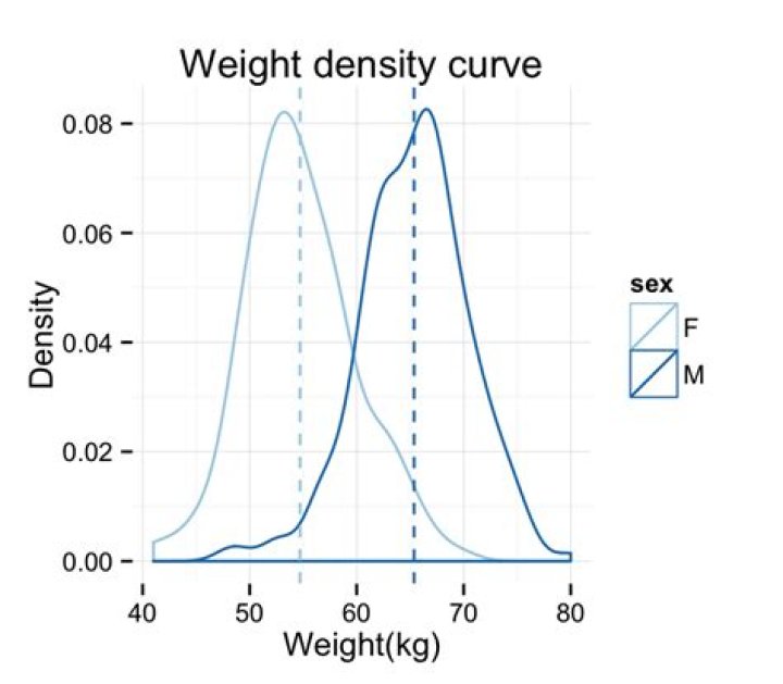 

In python (with matplotlib) the closest I got was with a simple histogram:

import matplotlib.pyplot as plt data = [1.5]*7 + [2.5]*2 + [3.5]*8 + [4.5]*3 + [5.5]*1 + [6.5]*8 plt.hist(data, bins=6) plt.show()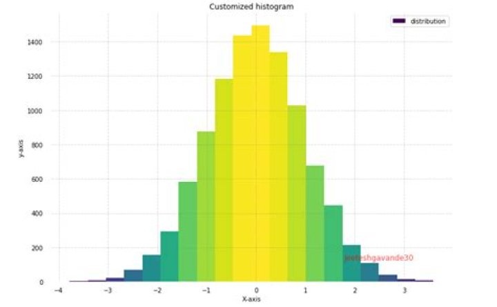 

I also tried the normed=True parameter but couldn't get anything other than trying to fit a gaussian to the histogram.

My latest attempts were around scipy.stats and gaussian_kde, following examples on the web, but I've been unsuccessful so far.

6 Answers

Five years later, when I Google "how to create a kernel density plot using python", this thread still shows up at the top!

Today, a much easier way to do this is to use seaborn, a package that provides many convenient plotting functions and good style management.

import numpy as np import seaborn as sns data = [1.5]*7 + [2.5]*2 + [3.5]*8 + [4.5]*3 + [5.5]*1 + [6.5]*8 sns.set_style('whitegrid') sns.kdeplot(np.array(data), bw=0.5) 

Sven has shown how to use the class gaussian_kde from Scipy, but you will notice that it doesn't look quite like what you generated with R. This is because gaussian_kde tries to infer the bandwidth automatically. You can play with the bandwidth in a way by changing the function covariance_factor of the gaussian_kde class. First, here is what you get without changing that function:

However, if I use the following code:

import matplotlib.pyplot as plt import numpy as np from scipy.stats import gaussian_kde data = [1.5]*7 + [2.5]*2 + [3.5]*8 + [4.5]*3 + [5.5]*1 + [6.5]*8 density = gaussian_kde(data) xs = np.linspace(0,8,200) density.covariance_factor = lambda : .25 density._compute_covariance() plt.plot(xs,density(xs)) plt.show() 

I get

which is pretty close to what you are getting from R. What have I done? gaussian_kde uses a changable function, covariance_factor to calculate its bandwidth. Before changing the function, the value returned by covariance_factor for this data was about .5. Lowering this lowered the bandwidth. I had to call _compute_covariance after changing that function so that all of the factors would be calculated correctly. It isn't an exact correspondence with the bw parameter from R, but hopefully it helps you get in the right direction.

Option 1:

Use pandas dataframe plot (built on top of matplotlib):

import pandas as pd data = [1.5]*7 + [2.5]*2 + [3.5]*8 + [4.5]*3 + [5.5]*1 + [6.5]*8 pd.DataFrame(data).plot(kind='density') # or pd.Series() 

Option 2:

Use distplot of seaborn:

import seaborn as sns data = [1.5]*7 + [2.5]*2 + [3.5]*8 + [4.5]*3 + [5.5]*1 + [6.5]*8 sns.distplot(data, hist=False) 

Maybe try something like:

import matplotlib.pyplot as plt import numpy from scipy import stats data = [1.5]*7 + [2.5]*2 + [3.5]*8 + [4.5]*3 + [5.5]*1 + [6.5]*8 density = stats.kde.gaussian_kde(data) x = numpy.arange(0., 8, .1) plt.plot(x, density(x)) plt.show() 

You can easily replace gaussian_kde() by a different kernel density estimate.

The density plot can also be created by using matplotlib: The function plt.hist(data) returns the y and x values necessary for the density plot (see the documentation ). Resultingly, the following code creates a density plot by using the matplotlib library:

import matplotlib.pyplot as plt dat=[-1,2,1,4,-5,3,6,1,2,1,2,5,6,5,6,2,2,2] a=plt.hist(dat,density=True) plt.close() plt.figure() plt.plot(a[1][1:],a[0]) 

This code returns the following density plot

You can do something like:

s = np.random.normal(2, 3, 1000) import matplotlib.pyplot as plt count, bins, ignored = plt.hist(s, 30, density=True) plt.plot(bins, 1/(3 * np.sqrt(2 * np.pi)) * np.exp( - (bins - 2)**2 / (2 * 3**2) ), linewidth=2, color='r') plt.show()