I am trying to plot a ROC curve to evaluate the accuracy of a prediction model I developed in Python using logistic regression packages. I have computed the true positive rate as well as the false positive rate; however, I am unable to figure out how to plot these correctly using matplotlib and calculate the AUC value. How could I do that?
14 Answers
Here are two ways you may try, assuming your model is an sklearn predictor:
import sklearn.metrics as metrics # calculate the fpr and tpr for all thresholds of the classification probs = model.predict_proba(X_test) preds = probs[:,1] fpr, tpr, threshold = metrics.roc_curve(y_test, preds) roc_auc = metrics.auc(fpr, tpr) # method I: plt import matplotlib.pyplot as plt plt.title('Receiver Operating Characteristic') plt.plot(fpr, tpr, 'b', label = 'AUC = %0.2f' % roc_auc) plt.legend(loc = 'lower right') plt.plot([0, 1], [0, 1],'r--') plt.xlim([0, 1]) plt.ylim([0, 1]) plt.ylabel('True Positive Rate') plt.xlabel('False Positive Rate') plt.show() # method II: ggplot from ggplot import * df = pd.DataFrame(dict(fpr = fpr, tpr = tpr)) ggplot(df, aes(x = 'fpr', y = 'tpr')) + geom_line() + geom_abline(linetype = 'dashed') or try
ggplot(df, aes(x = 'fpr', ymin = 0, ymax = 'tpr')) + geom_line(aes(y = 'tpr')) + geom_area(alpha = 0.2) + ggtitle("ROC Curve w/ AUC = %s" % str(roc_auc)) This is the simplest way to plot an ROC curve, given a set of ground truth labels and predicted probabilities. Best part is, it plots the ROC curve for ALL classes, so you get multiple neat-looking curves as well
import scikitplot as skplt import matplotlib.pyplot as plt y_true = # ground truth labels y_probas = # predicted probabilities generated by sklearn classifier skplt.metrics.plot_roc_curve(y_true, y_probas) plt.show() Here's a sample curve generated by plot_roc_curve. I used the sample digits dataset from scikit-learn so there are 10 classes. Notice that one ROC curve is plotted for each class.
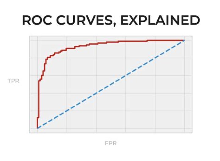
Disclaimer: Note that this uses the scikit-plot library, which I built.
10AUC curve For Binary Classification using matplotlib
from sklearn import svm, datasets from sklearn import metrics from sklearn.linear_model import LogisticRegression from sklearn.model_selection import train_test_split from sklearn.datasets import load_breast_cancer import matplotlib.pyplot as plt Load Breast Cancer Dataset
breast_cancer = load_breast_cancer() X = breast_cancer.data y = breast_cancer.target Split the Dataset
X_train, X_test, y_train, y_test = train_test_split(X,y,test_size=0.33, random_state=44) Model
clf = LogisticRegression(penalty='l2', C=0.1) clf.fit(X_train, y_train) y_pred = clf.predict(X_test) Accuracy
print("Accuracy", metrics.accuracy_score(y_test, y_pred)) AUC Curve
y_pred_proba = clf.predict_proba(X_test)[::,1] fpr, tpr, _ = metrics.roc_curve(y_test, y_pred_proba) auc = metrics.roc_auc_score(y_test, y_pred_proba) plt.plot(fpr,tpr,label="data 1, auc="+str(auc)) plt.legend(loc=4) plt.show() 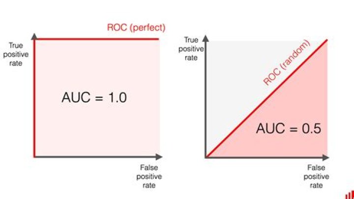
It is not at all clear what the problem is here, but if you have an array true_positive_rate and an array false_positive_rate, then plotting the ROC curve and getting the AUC is as simple as:
import matplotlib.pyplot as plt import numpy as np x = # false_positive_rate y = # true_positive_rate # This is the ROC curve plt.plot(x,y) plt.show() # This is the AUC auc = np.trapz(y,x) Here is python code for computing the ROC curve (as a scatter plot):
import matplotlib.pyplot as plt import numpy as np score = np.array([0.9, 0.8, 0.7, 0.6, 0.55, 0.54, 0.53, 0.52, 0.51, 0.505, 0.4, 0.39, 0.38, 0.37, 0.36, 0.35, 0.34, 0.33, 0.30, 0.1]) y = np.array([1,1,0, 1, 1, 1, 0, 0, 1, 0, 1,0, 1, 0, 0, 0, 1 , 0, 1, 0]) # false positive rate fpr = [] # true positive rate tpr = [] # Iterate thresholds from 0.0, 0.01, ... 1.0 thresholds = np.arange(0.0, 1.01, .01) # get number of positive and negative examples in the dataset P = sum(y) N = len(y) - P # iterate through all thresholds and determine fraction of true positives # and false positives found at this threshold for thresh in thresholds: FP=0 TP=0 for i in range(len(score)): if (score[i] > thresh): if y[i] == 1: TP = TP + 1 if y[i] == 0: FP = FP + 1 fpr.append(FP/float(N)) tpr.append(TP/float(P)) plt.scatter(fpr, tpr) plt.show() from sklearn import metrics import numpy as np import matplotlib.pyplot as plt y_true = # true labels y_probas = # predicted results fpr, tpr, thresholds = metrics.roc_curve(y_true, y_probas, pos_label=0) # Print ROC curve plt.plot(fpr,tpr) plt.show() # Print AUC auc = np.trapz(tpr,fpr) print('AUC:', auc) Based on multiple comments from stackoverflow, scikit-learn documentation and some other, I made a python package to plot ROC curve (and other metric) in a really simple way.
To install package : pip install plot-metric (more info at the end of post)
To plot a ROC Curve (example come from the documentation) :
Binary classification
Let's load a simple dataset and make a train & test set :
from sklearn.datasets import make_classification from sklearn.model_selection import train_test_split X, y = make_classification(n_samples=1000, n_classes=2, weights=[1,1], random_state=1) X_train, X_test, y_train, y_test = train_test_split(X, y, test_size=0.5, random_state=2) Train a classifier and predict test set :
from sklearn.ensemble import RandomForestClassifier clf = RandomForestClassifier(n_estimators=50, random_state=23) model = clf.fit(X_train, y_train) # Use predict_proba to predict probability of the class y_pred = clf.predict_proba(X_test)[:,1] You can now use plot_metric to plot ROC Curve :
from plot_metric.functions import BinaryClassification # Visualisation with plot_metric bc = BinaryClassification(y_test, y_pred, labels=["Class 1", "Class 2"]) # Figures plt.figure(figsize=(5,5)) bc.plot_roc_curve() plt.show() Result : 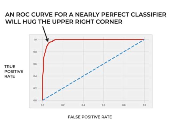
You can find more example of on the github and documentation of the package:
1The previous answers assume that you indeed calculated TP/Sens yourself. It's a bad idea to do this manually, it's easy to make mistakes with the calculations, rather use a library function for all of this.
the plot_roc function in scikit_lean does exactly what you need:
The essential part of the code is:
for i in range(n_classes): fpr[i], tpr[i], _ = roc_curve(y_test[:, i], y_score[:, i]) roc_auc[i] = auc(fpr[i], tpr[i]) You can also follow the offical documentation form scikit:
There is a library called metriculous that will do that for you:
$ pip install metriculous Let's first mock some data, this would usually come from the test dataset and the model(s):
import numpy as np def normalize(array2d: np.ndarray) -> np.ndarray: return array2d / array2d.sum(axis=1, keepdims=True) class_names = ["Cat", "Dog", "Pig"] num_classes = len(class_names) num_samples = 500 # Mock ground truth ground_truth = np.random.choice(range(num_classes), size=num_samples, p=[0.5, 0.4, 0.1]) # Mock model predictions perfect_model = np.eye(num_classes)[ground_truth] noisy_model = normalize( perfect_model + 2 * np.random.random((num_samples, num_classes)) ) random_model = normalize(np.random.random((num_samples, num_classes))) Now we can use metriculous to generate a table with various metrics and diagrams, including ROC curves:
import metriculous metriculous.compare_classifiers( ground_truth=ground_truth, model_predictions=[perfect_model, noisy_model, random_model], model_names=["Perfect Model", "Noisy Model", "Random Model"], class_names=class_names, one_vs_all_figures=True, # This line is important to include ROC curves in the output ).save_html("model_comparison.html").display() The ROC curves in the output: 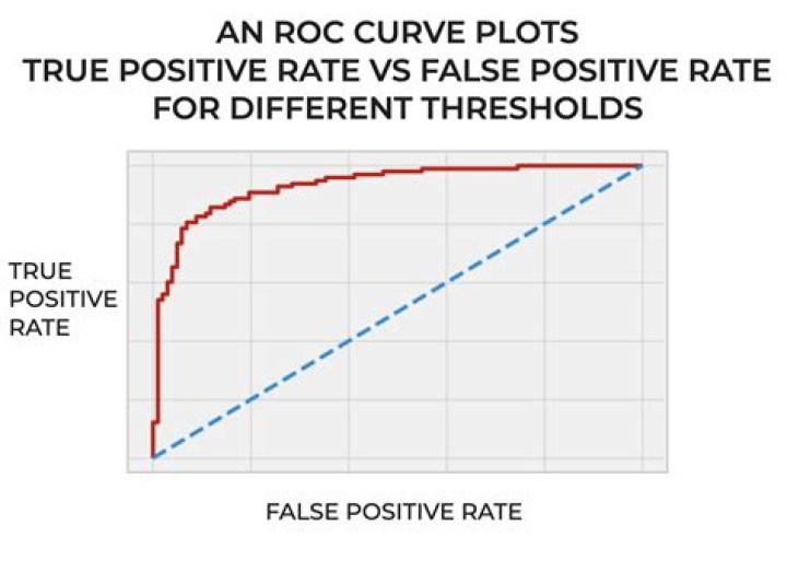
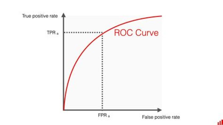
The plots are zoomable and draggable, and you get further details when hovering with your mouse over the plot:
I have made a simple function included in a package for the ROC curve. I just started practicing machine learning so please also let me know if this code has any problem!
Have a look at the github readme file for more details! :)
from sklearn.metrics import confusion_matrix, accuracy_score, roc_auc_score, roc_curve import matplotlib.pyplot as plt import seaborn as sns import numpy as np def plot_ROC(y_train_true, y_train_prob, y_test_true, y_test_prob): ''' a funciton to plot the ROC curve for train labels and test labels. Use the best threshold found in train set to classify items in test set. ''' fpr_train, tpr_train, thresholds_train = roc_curve(y_train_true, y_train_prob, pos_label =True) sum_sensitivity_specificity_train = tpr_train + (1-fpr_train) best_threshold_id_train = np.argmax(sum_sensitivity_specificity_train) best_threshold = thresholds_train[best_threshold_id_train] best_fpr_train = fpr_train[best_threshold_id_train] best_tpr_train = tpr_train[best_threshold_id_train] y_train = y_train_prob > best_threshold cm_train = confusion_matrix(y_train_true, y_train) acc_train = accuracy_score(y_train_true, y_train) auc_train = roc_auc_score(y_train_true, y_train) print 'Train Accuracy: %s ' %acc_train print 'Train AUC: %s ' %auc_train print 'Train Confusion Matrix:' print cm_train fig = plt.figure(figsize=(10,5)) ax = fig.add_subplot(121) curve1 = ax.plot(fpr_train, tpr_train) curve2 = ax.plot([0, 1], [0, 1], color='navy', linestyle='--') dot = ax.plot(best_fpr_train, best_tpr_train, marker='o', color='black') ax.text(best_fpr_train, best_tpr_train, s = '(%.3f,%.3f)' %(best_fpr_train, best_tpr_train)) plt.xlim([0.0, 1.0]) plt.ylim([0.0, 1.0]) plt.xlabel('False Positive Rate') plt.ylabel('True Positive Rate') plt.title('ROC curve (Train), AUC = %.4f'%auc_train) fpr_test, tpr_test, thresholds_test = roc_curve(y_test_true, y_test_prob, pos_label =True) y_test = y_test_prob > best_threshold cm_test = confusion_matrix(y_test_true, y_test) acc_test = accuracy_score(y_test_true, y_test) auc_test = roc_auc_score(y_test_true, y_test) print 'Test Accuracy: %s ' %acc_test print 'Test AUC: %s ' %auc_test print 'Test Confusion Matrix:' print cm_test tpr_score = float(cm_test[1][1])/(cm_test[1][1] + cm_test[1][0]) fpr_score = float(cm_test[0][1])/(cm_test[0][0]+ cm_test[0][1]) ax2 = fig.add_subplot(122) curve1 = ax2.plot(fpr_test, tpr_test) curve2 = ax2.plot([0, 1], [0, 1], color='navy', linestyle='--') dot = ax2.plot(fpr_score, tpr_score, marker='o', color='black') ax2.text(fpr_score, tpr_score, s = '(%.3f,%.3f)' %(fpr_score, tpr_score)) plt.xlim([0.0, 1.0]) plt.ylim([0.0, 1.0]) plt.xlabel('False Positive Rate') plt.ylabel('True Positive Rate') plt.title('ROC curve (Test), AUC = %.4f'%auc_test) plt.savefig('ROC', dpi = 500) plt.show() return best_threshold A sample roc graph produced by this code
2When you need the probabilities as well... The following gets the AUC value and plots it all in one shot.
from sklearn.metrics import plot_roc_curve plot_roc_curve(m,xs,y) When you have the probabilities... you can't get the auc value and plots in one shot. Do the following:
from sklearn.metrics import roc_curve fpr,tpr,_ = roc_curve(y,y_probas) plt.plot(fpr,tpr, label='AUC = ' + str(round(roc_auc_score(y,m.oob_decision_function_[:,1]), 2))) plt.legend(loc='lower right') A new open-source I help maintain have many ways to test model performance. to see ROC curve you can do:
from deepchecks.checks import RocReport from deepchecks import Dataset RocReport().run(Dataset(df, label='target'), model) And the result looks like this:  A more elaborate example of RocReport can be found here
In my code, I have X_train and y_train and classes are 0 and 1. The clf.predict_proba() method computes probabilities for both classes for every data point. I compare the probability of class1 with different values of threshold.
probability = clf.predict_proba(X_train) def plot_roc(y_train, probability): threshold_values = np.linspace(0,1,100) #Threshold values range from 0 to 1 FPR_list = [] TPR_list = [] for threshold in threshold_values: #For every value of threshold y_pred = [] #Classify every data point in the test set #prob is an array consisting of 2 values - Probability of datapoint in Class0 and Class1. for prob in probability: if ((prob[1])<threshold): #Prob of class1 (positive class) y_pred.append(0) continue elif ((prob[1])>=threshold): y_pred.append(1) #Plot Confusion Matrix and Obtain values of TP, FP, TN, FN c_m = confusion_matrix(y, y_pred) TN = c_m[0][0] FP = c_m[0][1] FN = c_m[1][0] TP = c_m[1][1] FPR = FP/(FP + TN) #Obtain False Positive Rate TPR = TP/(TP + FN) #Obtain True Positive Rate FPR_list.append(FPR) TPR_list.append(TPR) fig = plt.figure() plt.plot(FPR_list, TPR_list) plt.ylabel('TPR') plt.xlabel('FPR') plt.show()