I have some data that I want to fit so I can make some estimations for the value of a physical parameter given a certain temperature.
I used numpy.polyfit for a quadratic model, but the fit isn't quite as nice as I'd like it to be and I don't have much experience with regression.
I have included the scatter plot and the model provided by numpy: S vs Temperature; blue dots are experimental data, black line is the model
The x axis is temperature (in C) and the y axis is the parameter, which we'll call S. This is experimental data, but in theory S should tends towards 0 as temperature increases and reach 1 as temperature decreases.
My question is: How can I fit this data better? What libraries should I use, what kind of function might approximate this data better than a polynomial, etc?
I can provide code, coefficients of the polynomial, etc, if it's helpful.
Here is a Dropbox link to my data. (Somewhat important note to avoid confusion, although it won't change the actual regression, the temperature column in this data set is Tc - T, where Tc is the transition temperature (40C). I converted this using pandas into T by calculating 40 - x).
27 Answers
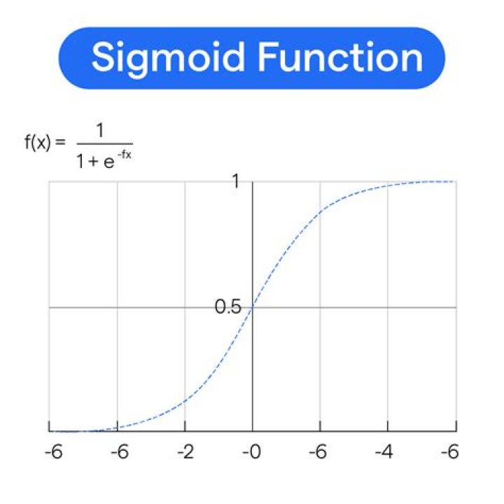
This example code uses an equation that has two shape parameters, a and b, and an offset term (that does not affect curvature). The equation is "y = 1.0 / (1.0 + exp(-a(x-b))) + Offset" with parameter values a = 2.1540318329369712E-01, b = -6.6744890642157646E+00, and Offset = -3.5241299859669645E-01 which gives an R-squared of 0.988 and an RMSE of 0.0085.
The example contains your posted data with Python code for fitting and graphing, with automatic initial parameter estimation using the scipy.optimize.differential_evolution genetic algorithm. The scipy implementation of Differential Evolution uses the Latin Hypercube algorithm to ensure a thorough search of parameter space, and this requires bounds within which to search - in this example code, these bounds are based on the maximum and minimum data values.
import numpy, scipy, matplotlib import matplotlib.pyplot as plt from scipy.optimize import curve_fit from scipy.optimize import differential_evolution import warnings xData = numpy.array([19.1647, 18.0189, 16.9550, 15.7683, 14.7044, 13.6269, 12.6040, 11.4309, 10.2987, 9.23465, 8.18440, 7.89789, 7.62498, 7.36571, 7.01106, 6.71094, 6.46548, 6.27436, 6.16543, 6.05569, 5.91904, 5.78247, 5.53661, 4.85425, 4.29468, 3.74888, 3.16206, 2.58882, 1.93371, 1.52426, 1.14211, 0.719035, 0.377708, 0.0226971, -0.223181, -0.537231, -0.878491, -1.27484, -1.45266, -1.57583, -1.61717]) yData = numpy.array([0.644557, 0.641059, 0.637555, 0.634059, 0.634135, 0.631825, 0.631899, 0.627209, 0.622516, 0.617818, 0.616103, 0.613736, 0.610175, 0.606613, 0.605445, 0.603676, 0.604887, 0.600127, 0.604909, 0.588207, 0.581056, 0.576292, 0.566761, 0.555472, 0.545367, 0.538842, 0.529336, 0.518635, 0.506747, 0.499018, 0.491885, 0.484754, 0.475230, 0.464514, 0.454387, 0.444861, 0.437128, 0.415076, 0.401363, 0.390034, 0.378698]) def func(x, a, b, Offset): # Sigmoid A With Offset from zunzun.com return 1.0 / (1.0 + numpy.exp(-a * (x-b))) + Offset # function for genetic algorithm to minimize (sum of squared error) def sumOfSquaredError(parameterTuple): warnings.filterwarnings("ignore") # do not print warnings by genetic algorithm val = func(xData, *parameterTuple) return numpy.sum((yData - val) ** 2.0) def generate_Initial_Parameters(): # min and max used for bounds maxX = max(xData) minX = min(xData) maxY = max(yData) minY = min(yData) parameterBounds = [] parameterBounds.append([minX, maxX]) # search bounds for a parameterBounds.append([minX, maxX]) # search bounds for b parameterBounds.append([0.0, maxY]) # search bounds for Offset # "seed" the numpy random number generator for repeatable results result = differential_evolution(sumOfSquaredError, parameterBounds, seed=3) return result.x # generate initial parameter values geneticParameters = generate_Initial_Parameters() # curve fit the test data fittedParameters, pcov = curve_fit(func, xData, yData, geneticParameters) print('Parameters', fittedParameters) modelPredictions = func(xData, *fittedParameters) absError = modelPredictions - yData SE = numpy.square(absError) # squared errors MSE = numpy.mean(SE) # mean squared errors RMSE = numpy.sqrt(MSE) # Root Mean Squared Error, RMSE Rsquared = 1.0 - (numpy.var(absError) / numpy.var(yData)) print('RMSE:', RMSE) print('R-squared:', Rsquared) ########################################################## # graphics output section def ModelAndScatterPlot(graphWidth, graphHeight): f = plt.figure(figsize=(graphWidth/100.0, graphHeight/100.0), dpi=100) axes = f.add_subplot(111) # first the raw data as a scatter plot axes.plot(xData, yData, 'D') # create data for the fitted equation plot xModel = numpy.linspace(min(xData), max(xData)) yModel = func(xModel, *fittedParameters) # now the model as a line plot axes.plot(xModel, yModel) axes.set_xlabel('X Data') # X axis data label axes.set_ylabel('Y Data') # Y axis data label plt.show() plt.close('all') # clean up after using pyplot graphWidth = 800 graphHeight = 600 ModelAndScatterPlot(graphWidth, graphHeight) I would suggest checking out scipy. They have a non-linear optimizer for fitting data to arbitrary functions. See the documentation for scipy.optimize.curve_fit here. Be aware that the more complex the function, the longer it will take to fit.
For non-linear regression problem, you could try SVR(), KNeighborsRegressor() or DecisionTreeRegression() from sklearn, and compare the model performance on the test set.
In Scikit Learn, you can use Polynomial Features to first transform your training data to have more degrees of freedom. After that, you can use Ridge Regression to fit your training data.
Here are a few options for creating a mathematical expression from your data:
- Nonlinear regression adjusts parameters in a single equation
- Interpolation such as linear or cubic-spline
- Empirical regression such as deep learning
I created a script with Python gekko to demonstrate each of these.
from gekko import GEKKO import numpy as np import matplotlib.pyplot as plt xData = np.array([19.1647,18.0189,16.955,15.7683,14.7044,13.6269,12.604,\ 11.4309,10.2987,9.23465,8.1844,7.89789,7.62498,7.36571,\ 7.01106,6.71094,6.46548,6.27436,6.16543,6.05569,5.91904,\ 5.78247,5.53661,4.85425,4.29468,3.74888,3.16206,2.58882,\ 1.93371,1.52426,1.14211,0.719035,0.377708,0.0226971,\ -0.223181,-0.537231,-0.878491,-1.27484,-1.45266,-1.57583,\ -1.61717]) yData = np.array([0.644557,0.641059,0.637555,0.634059,0.634135,0.631825,\ 0.631899,0.627209,0.622516,0.617818,0.616103,0.613736,\ 0.610175,0.606613,0.605445,0.603676,0.604887,0.600127,\ 0.604909,0.588207,0.581056,0.576292,0.566761,0.555472,\ 0.545367,0.538842,0.529336,0.518635,0.506747,0.499018,\ 0.491885,0.484754,0.47523,0.464514,0.454387,0.444861,\ 0.437128,0.415076,0.401363,0.390034,0.378698]) m = GEKKO(remote=False) # nonlinear regression a,b,c = m.Array(m.FV,3,value=0,lb=-10,ub=10) x = m.MV(xData); y = m.CV(yData) a.STATUS=1; b.STATUS=1; c.STATUS=1; y.FSTATUS=1 m.Equation(y==1.0/(1.0+m.exp(-a*(x-b)))+c) # cubic spline z = m.Var() m.cspline(x,z,xData,yData,True) m.options.IMODE = 2; m.options.EV_TYPE = 2 m.solve() # stats (from other answer) absError = y.value - yData SE = np.square(absError) # squared errors MSE = np.mean(SE) # mean squared errors RMSE = np.sqrt(MSE) # Root Mean Squared Error, RMSE Rsquared = 1.0 - (np.var(absError) / np.var(yData)) print('RMSE:', RMSE) print('R-squared:', Rsquared) print('Parameters', a.value[0], b.value[0], c.value[0]) # deep learning from gekko import brain b = brain.Brain() b.input_layer(1) b.layer(linear=1) b.layer(tanh=2) b.layer(linear=1) b.output_layer(1) b.learn(xData,yData,obj=1,disp=False) # train xp = np.linspace(min(xData),max(xData),100) w = b.think(xp) # predict plt.plot(xData,yData,'k.',label='data') plt.plot(x.value,y.value,'r:',lw=3,label=r'$1/(1+exp(-a(x-b)+c)$') plt.plot(x.value,z.value,'g--',label='c-spline') plt.plot(xp,w[0],'b-.',label='deep learning') plt.legend(); plt.show() The regression results are:
RMSE: 0.008428738368115708 R-squared: 0.988622263162808 Parameters 0.2154031832 -6.6744890468 -0.3524129987 The deep learning is similar to the single regression equation but the layers and activation functions are more easily adjusted than creating an equation form yourself. The advantage of the single equation is that it may extrapolate better than a machine learned model. Interpolation such as a piecewise linear or cubic-spline function may be good if you don't need to extrapolate and there is little variability in individual data points. Here is more information that I created on regression and interpolation with more examples in the Jupyter notebooks.
A more robust nonlinear optimization can be obtained by mitigating the leverage of outliers using sublinear loss function like soft l1.
Also, any domain knowledge of the solution bound may avoid the use of the genetic generation of initial parameters. Especially relevant if the features have not been scaled.
Try a support vector machine with a polynomial kernel.
With scikit-learn, fitting a model can be as simple as:
from sklearn.svm import SVC #... load the data into X,y model = SVC(kernel='poly') model.fit(X,y) #plot the model...